Sampling Distribution of the Sample Mean Clearly Explained
What is Sampling Distribution of the Sample Mean?
We use sample mean as one of the measures of summary of variables in a study. In other words, sample mean is the average of the values observed. Lets imagine you conduct the same study with same sample size again and again and calculate sample mean in each case. Frequency distribution of sample means obtained from those repeated studies is called sampling distribution of the mean. It can be displayed using histogram or density curve.
For example, you run a study of sample size 12000 and replicate it 1000 times. Assume our data is normally distributed for simulation purposes. We will calculate 1000 sample means and show the distribution of those means using histogram overlayed with density curve as described below.
#set libraries
library(tidyverse)
## -- Attaching packages --------------------------------------------------------- tidyverse 1.2.1 --## v ggplot2 3.1.0 v purrr 0.3.1
## v tibble 2.0.1 v dplyr 0.8.0.1
## v tidyr 0.8.3 v stringr 1.4.0
## v readr 1.3.1 v forcats 0.4.0## -- Conflicts ------------------------------------------------------------ tidyverse_conflicts() --
## x dplyr::filter() masks stats::filter()
## x dplyr::lag() masks stats::lag()library(ggplot2)
library(dplyr)#replicate a study of sample size 12000 1000 times and calculate sample mean of each of those studies
set.seed(1431)
sample_avg = rep(NA, 1000) #replicate NA 1000 times
for (i in 1:1000){
sample_avg[i]= mean(rnorm(12000))
}
#sample_avg<- as.integer(sample_avg)
#change the distribution of sample mean to data frame
sample<-as.data.frame(sample_avg)
#create histogram of sampling distribution of the sample mean overlayed with density curve
hist<- ggplot(sample, aes(x=sample_avg)) +
geom_histogram(aes(y=..density..)) + geom_density() +
labs(x="Sample Average",y="Density") + ggtitle("Histogram showing sampling distribution of the sample mean")
hist## `stat_bin()` using `bins = 30`. Pick better value with `binwidth`.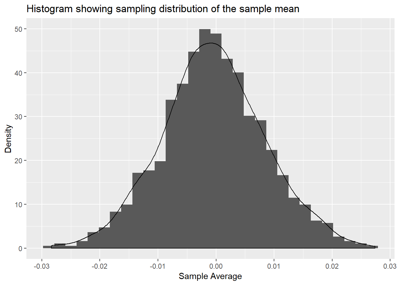
This idea of sampling distribution is the fundamental concept based on which statistical inferences are made in frequentist Statistics. We will look at it more closely how it applies to one of the most important ideas in statistics called ‘Central Limit Theorem’ in another post.
One thing that comes to mind after going through this explanation is that its not easy to repeat studies to estimate sampling distribution of sample mean in practice. We will have to use statistical techniques that would be able to estimate sampling distribution of the mean from a single random sample. We will discuss more about this in later posts in details.