Confidence Interval
How do you explain confidence intervals intuitively?
In any study,We all know we want to test our hypothesis to see if there is any difference between our assigned groups using some kind of experiment. As a common rule, point estimate is calculated as the difference in means between two groups and 95 % confidence interval is reported as a means of quantifying uncertainty associated with that estimate.
When people hear about 95% confidence interval, they mistakenly interpret it as the interval with 95% chance of containing true population parameter we are trying to estimate. This is entirely a wrong way to think about confidence interval. Let me make this clear with a simulation example.
Textbook definition of 95% confidence interval tells us that if we repeatedly conduct experiments of sample size n and calculate confidence interval in each case, 95 % of those intervals would contain the population parameter we are trying to estimate.
Assume an experiment where we want to find out the effect of a treatment (Active vs Control) on our outcome. Lets assume for our outcome simulation We have following population parameters. It means we know true population effect here since we created this for simulation. It is always unknown in real world.
- true population effect delta= 200 (true difference in mean outcome between Active and control group)
- standard deviation = 100
- Sample size = 200
- Number of trials repeated with this sample size = 100
set.seed(148)
n <- 200
sigma<-100
delta<-200
# Store means, upper and lower intervals from 100 trials
means<-c()
upper<-c()
lower<-c()

for (i in 1:100) {
  #Simulate a normal distribution using above parameters
  x<-rnorm(n,delta,sigma)
  means[i]<-mean(x)
  lower[i]<-means[i]-1.96*sigma/sqrt(n)
  upper[i]<- means[i]+1.96*sigma/sqrt(n)

}

# change to dataframe
means_frame<- as.data.frame(means)
id<-rownames(means_frame)
id<-as.numeric(id)
means_list<-cbind(means_frame,id)

upp_lower<-as.data.frame(cbind(lower,upper))
#plot 95% confidence interval for each estimate
true_value<-ifelse (lower >= 200 & upper >= 200 ,1,0)
true<-as.data.frame(true_value)
#Combine everything into one dataset
all<-cbind(upp_lower,true, means_list)
g<-ggplot(all,aes(id,means,color=factor(true_value,labels=c("Includes true effect","Excludes true effect")))) +
geom_errorbar(aes(ymin=lower,ymax=upper)) +
geom_line() +
geom_point() +
scale_x_continuous(limits=c(0,100)) +
labs(x="Number of Trials",y="Confidence limit",color="Confidence") +
geom_hline(yintercept=200,color="black",linetype="dashed",size=0.5)
g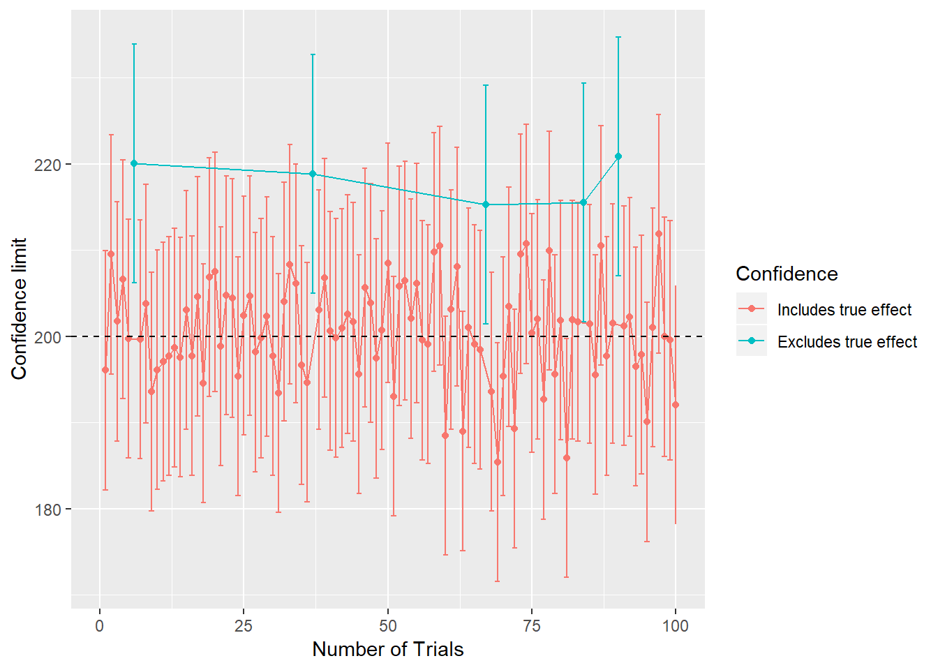
Here, as stated in the definition of 95% confidence interval we calculated confidence intervals for 100 trials with same sample size. As expected we clearly see from above figure (indicated by green dots and error bars), 5 trials out of 100 didn’t have confidence limit that contain true population effect of 200. Remaining 95 intervals contain true population effect.
It is important to notice that we will never know true population effect in practice. Some intervals will contain true value whereas some won’t. We cannot tell which contain the true effect. However, provided that we know nothing about true effect, we can assign a probability for the confidence interval being included in our analysis. Looking at the figure above we can say 95 out of 100 i.e. 95% of the intervals cover true value.