Central Limit Theorem
What is Central Limit Theorem?
Textbook definition of Central Limit Theorem states that “As sample size increases, the sampling distribution of the mean for an independent identically distributed variable will approximately resemble that of normal distribution regardless of its distribution”.
This definition of CLT needs some breakdown into simpler parts. First of all, a random variable can have different probability distribution. It could be right, left skewed or uniformly distributed etc.. However, if that variable has sufficient enough sample size, its distribution approximates normal distribution irrespective of the probability distribution. We will explore this key idea using a series of simulation examples.
#set libraries
library(tidyverse)
## -- Attaching packages --------------------------------------------------------- tidyverse 1.2.1 --## v ggplot2 3.1.0 v purrr 0.3.1
## v tibble 2.0.1 v dplyr 0.8.0.1
## v tidyr 0.8.3 v stringr 1.4.0
## v readr 1.3.1 v forcats 0.4.0## -- Conflicts ------------------------------------------------------------ tidyverse_conflicts() --
## x dplyr::filter() masks stats::filter()
## x dplyr::lag() masks stats::lag()library(ggplot2)
library(dplyr)# Let's look at a right skewed (negative binomial distribution)
set.seed(1536)
#this gives us a set of random numbers that follow negative binomial distribution with a sample size of 100
neg_binom<-rnbinom(100,30,0.3)
neg_binom1<-as.data.frame(neg_binom)
#plot histogram and density curve
hist<- ggplot(neg_binom1, aes(x=neg_binom)) +
geom_histogram(aes(y=..density..),bins=20) + geom_density() +
labs(x="X",y="Density") + ggtitle("Right Skewed negative binomial distribution")
hist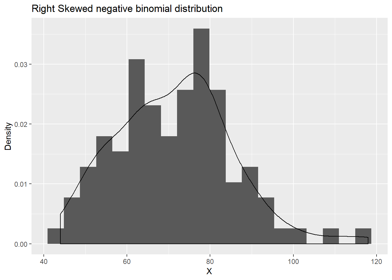
If we increase sample size sufficiently enough, we will see the distibution of the variable X resembles to that of normal distribution. This means we will acheive a symmetrical distribution of this right skewed variable if we have larger enough sample size. Lets see if we can show this in an example:
# Let's take the same negative binomial distribution with large sample size

set.seed(1546)
#this gives us a set of random numbers that follow negative binomial distribution with a sample size of 10000
neg_binom<-rnbinom(10000,30,0.3)
neg_binom1<-as.data.frame(neg_binom)

#plot histogram and density curve
hist<- ggplot(neg_binom1, aes(x=neg_binom)) +
  geom_histogram(aes(y=..density..),bins=20) + geom_density() +
  labs(x="X",y="Density") + ggtitle("Normal Distribution obtained using larger sample size")
hist
Here, once we sufficiently increase the number of samples, the right skewed binomial distribution with same parameters resembles normal distribution. As we can clearly see from the figure that concentration of the values generated is around the center which is mean of the distribution approximating normal distribution.
You can take any skewed family of distribution and repeat above procedures of simulation with larger sample size and you will get the distribution that approximates normal distribution. This concept of central limit theorem has broader implications in the field of statistical inferences. I will expand on this in more details in future posts.